Machine Learning (ML) is a subset of Artificial Intelligence (AI) that focuses on developing algorithms that enable computers to learn from and make decisions based on data. Rather than being explicitly programmed to perform a task, ML algorithms build a model based on sample inputs to make predictions or decisions without human intervention. This learning process involves the use of statistical techniques to identify patterns and relationships within the data, thereby enabling the machine to improve its performance over time with more data.

Artificial Intelligence, a term more people are familiar with, encompasses a broader range of techniques, including rule-based systems, natural language processing, and robotics, with the goal of creating systems that can perform tasks typically requiring human intelligence. Machine Learning is a crucial part of AI as it provides the ability to adapt and improve autonomously. In essence, while AI aims to simulate intelligent behaviour, ML is the method by which this intelligence is achieved through data-driven learning, which is perfect for trading and financial markets.

Random Forest Model in Trading Technical Analysis

I’ve written about many AI and ML models and techniques that can be used with trading and financial markets. My last article, “AI Reinforcement Learning with OpenAI’s Gym” may be of interest. I also recommend checking out EODHD API’s Medium page. I use their APIs to provide the financial data to train my models. It’s really easy to use and I also wrote a Python library for them that simplifies data retrieval.

In this article I want to introduce and demonstrate the Random Forest model. The model is a learning method used for classification and regression tasks. It operates by constructing multiple decision trees during training and outputting the mode of the classes (for classification) or mean prediction (for regression) of the individual trees. The ensemble of trees (the forest) mitigates the risk of overfitting to the training data, providing robust and accurate predictions.

In trading technical analysis, the Random Forest model can be particularly useful due to its ability to handle large amounts of data and complex patterns. For example, a trader might use Random Forest to predict stock price movements based on historical price data, volume, and other technical indicators such as moving averages and relative strength index (RSI). By training the model on historical data, it can learn the intricate relationships between these indicators and future price movements.

For instance, suppose a trader uses a dataset containing daily stock or cryptocurrency prices, volume, and technical indicators over the past five years. The Random Forest model can be trained to predict the likelihood of the price increasing or decreasing the next day. By inputting the current day’s data, the model provides a probability that can inform the trader’s decision to buy or sell, potentially improving trading outcomes by leveraging the model’s pattern recognition capabilities. This method not only enhances predictive accuracy but also helps in managing risks by providing a probabilistic assessment of future price movements.

Let’s look at a practical example…

The first step is we will need to retrieve some data to work with. For interest sake, I’m going to use Bitcoin’s daily data. What I like about EODHD APIs is it’s fast with little to no retrieval limits. The code below retrieves 1999 days of data.

from eodhd import APIClient
import config as cfg

api = APIClient(cfg.API_KEY)

def get_ohlc_data():
# df = api.get_historical_data("GSPC.INDX", "d", results=2000)
df = api.get_historical_data("BTC-USD.CC", "d", results=2000)
return df

if __name__ == "__main__":
df = get_ohlc_data()
print(df)

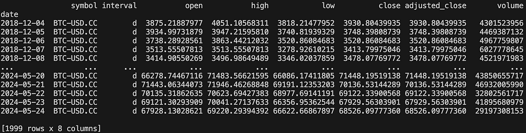Screenshot by Author

What I want to do now is add some technical indicators. This really is up to you and part of the fun of experimenting. I’m going to add SMA50, SMA200, MACD, RSI14, and VROC. You can add whatever you prefer here.

def calculate_sma(data, window):
return data.rolling(window=window).mean()

def calculate_macd(data, short_window=12, long_window=26, signal_window=9):
short_ema = data.ewm(span=short_window, adjust=False).mean()
long_ema = data.ewm(span=long_window, adjust=False).mean()
macd = short_ema - long_ema
signal_line = macd.ewm(span=signal_window, adjust=False).mean()
return macd, signal_line

def calculate_rsi(data, window=14):
delta = data.diff(1)
gain = (delta.where(delta > 0, 0)).rolling(window=window).mean()
loss = (-delta.where(delta < 0, 0)).rolling(window=window).mean()
rs = gain / loss
rsi = 100 - (100 / (1 + rs))
return rsi

def calculate_vroc(volume, window=14):
vroc = ((volume.diff(window)) / volume.shift(window)) * 100
return vroc

if __name__ == "__main__":
df = get_ohlc_data()

df["sma50"] = calculate_sma(df["close"], 50)
df["sma200"] = calculate_sma(df["close"], 200)
df["macd"], df["signal"] = calculate_macd(df["close"])
df["rsi14"] = calculate_rsi(df["close"])
df["vroc14"] = calculate_vroc(df["volume"])

df.dropna(inplace=True)

print(df)

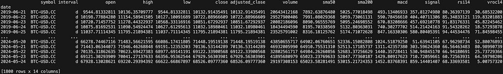Screenshot by Author

This should be self explanatory, but I want to point out something important. You will see that I drop non-numeric rows at the end “dropna”. This is really important as ML models can only handle numeric values. I’m now left with 1800 days of interesting data to work with.

Normalisation and Scaling

If you have read my other articles you will notice that I almost always normalise and scale my data between 0 and 1. This is sort of an exception to the rule. In general, scaling is not a strict requirement when using Random Forests because they are based on decision trees, which are not sensitive to the scale of the input features. However, scaling can still be beneficial in some scenarios, particularly when integrating Random Forests into a pipeline with other algorithms that do require scaling. Additionally, if you plan to interpret feature importances, having scaled data can sometimes make these interpretations more straightforward. For this example I’m not going to run the data through a scaler. You may want to do it, and if you do, I’ve explained how to do it in my previous articles. If you need help, just ask in the comments.

Model Training

Training an ML model is actually very straightforward and requires very little code thanks to some essential libraries. You will want to install “scikit-learn” using PIP.

% python3 -m pip install scikit-learn -U

What you will want to do is split your data into a train set and a test set. I almost always use a 70/30 or 80/20 split. I’ll use a 80/20 split here.

# include these library imports at the top of your file

from sklearn.model_selection import train_test_split
from sklearn.ensemble import RandomForestRegressor
from sklearn.metrics import mean_absolute_error, mean_squared_error, r2_score

# put this in your main at the end

features = [
"open",
"high",
"low",
"volume",
"sma50",
"sma200",
"macd",
"signal",
"rsi14",
"vroc14",
]
X = df[features]
y = df["close"]
X_train, X_test, y_train, y_test = train_test_split(
X, y, test_size=0.2, random_state=42
)

And you can see that the shape of the X_train, X_test, y_train, and y_test looks like this.

print(X_train.shape, X_test.shape, y_train.shape, y_test.shape)

(1440, 10) (360, 10) (1440,) (360,)

This is all you need to do to fit your model.

rf = RandomForestRegressor(n_estimators=100, random_state=42)
rf.fit(X_train, y_train)Making Predictionsy_train_pred = rf.predict(X_train)
y_test_pred = rf.predict(X_test)Visualisation of the Predictions

Install the “matplotlib” and “seaborn” libraries using PIP.

% python3 -m pip install matplotlib seaborn -U

Include the libraries in your code.

import matplotlib.pyplot as plt
import seaborn as sns

Scatter Plot of Actual vs. Predicted Values

plt.figure(figsize=(14, 7))

plt.subplot(1, 2, 1)
plt.scatter(y_train, y_train_pred, alpha=0.3)
plt.xlabel("Actual Close Price (Train)")
plt.ylabel("Predicted Close Price (Train)")
plt.title("Actual vs. Predicted Close Price (Training Set)")
plt.plot([y_train.min(), y_train.max()], [y_train.min(), y_train.max()], "r--")

plt.subplot(1, 2, 2)
plt.scatter(y_test, y_test_pred, alpha=0.3)
plt.xlabel("Actual Close Price (Test)")
plt.ylabel("Predicted Close Price (Test)")
plt.title("Actual vs. Predicted Close Price (Testing Set)")
plt.plot([y_test.min(), y_test.max()], [y_test.min(), y_test.max()], "r--")

plt.tight_layout()
plt.show()

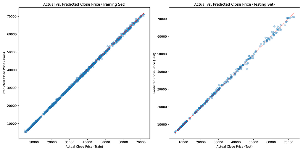Screenshot by Author

Line Plot of Actual vs. Predicted Values Over Time

plt.figure(figsize=(14, 7))

plt.plot(y_test.index, y_test, label="Actual Close Price")
plt.plot(y_test.index, y_test_pred, label="Predicted Close Price")
plt.xlabel("Date")
plt.ylabel("Close Price")
plt.title("Actual vs. Predicted Close Price Over Time (Testing Set)")
plt.legend()
plt.show()

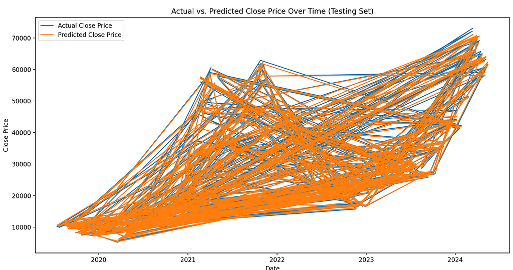Screenshot by AuthorEvaluating the Performance of the Model

An important task to perform when working with any AI/ML model is to evaluate the performance. This can be very useful when comparing models. There may be more, but the ones I’ve always used are Mean Absolute Error (MAE), Mean Squared Error (MSE), and the R-squared score (R²). They seem to be the most common.

train_mae = mean_absolute_error(y_train, y_train_pred)
test_mae = mean_absolute_error(y_test, y_test_pred)
train_mse = mean_squared_error(y_train, y_train_pred)
test_mse = mean_squared_error(y_test, y_test_pred)
train_r2 = r2_score(y_train, y_train_pred)
test_r2 = r2_score(y_test, y_test_pred)

print(f"Training MAE: {train_mae}")
print(f"Testing MAE: {test_mae}")
print(f"Training MSE: {train_mse}")
print(f"Testing MSE: {test_mse}")
print(f"Training R²: {train_r2}")
print(f"Testing R²: {test_r2}")

The result for my model looks like this:

Training MAE: 149.95774584583577
Testing MAE: 375.66243670875343
Training MSE: 59806.0910378797
Testing MSE: 402962.34869884106
Training R²: 0.9998008096169744
Testing R²: 0.9987438463433689

Mean Absolute Error (MAE):

Training MAE: 149.96
Testing MAE: 375.66

MAE measures the average absolute errors between the predicted and actual values. It provides a straightforward measure of how far off predictions are on average.

A lower MAE indicates better model performance.
Here, the Training MAE is significantly lower than the Testing MAE, suggesting that the model performs better on the training data compared to the testing data.

Mean Squared Error (MSE):

Training MSE: 59806.09
Testing MSE: 402962.35

MSE measures the average squared errors between the predicted and actual values. It penalises larger errors more than MAE, making it sensitive to outliers.

A lower MSE indicates better model performance.
Similar to MAE, the Training MSE is much lower than the Testing MSE, indicating better performance on the training data.

R-squared (R²):

Training R²: 0.9998
Testing R²: 0.9987

R² measures the proportion of the variance in the dependent variable that is predictable from the independent variables. It ranges from 0 to 1, where 1 indicates perfect prediction.

A higher R² indicates better model performance.
Both Training and Testing R² values are very high, close to 1, indicating that the model explains almost all the variance in the data for both training and testing sets.

So what does this actually mean and why is it important?

The model performs exceptionally well on the training data, as indicated by the low Training MAE and MSE and the high Training R². This suggests that the model has learned the patterns in the training data very well.
The model also performs very well on the testing data, as indicated by the high Testing R². However, the Testing MAE and MSE are higher compared to the training metrics. This discrepancy suggests some degree of overfitting, where the model might be capturing noise in the training data that does not generalise well to the unseen testing data.

The significant difference between the training and testing errors (both MAE and MSE) suggests that the model may be slightly overfitting the training data. Overfitting occurs when a model learns the training data too well, including its noise and outliers, which negatively impacts its performance on new, unseen data.

What could we do to improve this?

Regularisation: We can consider using techniques to reduce overfitting, such as limiting the maximum depth of the trees, reducing the number of trees, or using other regularisation methods.

Cross-Validation: We can perform cross-validation to ensure that the model’s performance is consistent across different subsets of the data.

Feature Engineering: We can re-evaluate the selected features and possibly introduce new features or reduce the number of features to improve model generalisability. As I explained in the beginning of the article, I just selected some random technical indicators for my tutorial. There could be some interesting features that could be included or swapped out. Maybe percentage change could be one to look at.

Hyperparameter Tuning: We can optimise the hyperparameters of the Random Forest model to balance bias and variance, potentially improving performance on the testing data.

These steps can help in achieving a better balance between training and testing performance, leading to a more robust and generalisable model. I don’t necessarily think we have a huge problem and this is just a tutorial. I just wanted to give you some food for thought about what you can do when trying this out yourself.

Here is some code to help you get started…

# update this import at the top

from sklearn.model_selection import train_test_split, cross_val_score, GridSearchCV

# modify the mode in your main

param_grid = {
"n_estimators": [50, 100, 200],
"max_depth": [10, 20, 30, None],
"min_samples_split": [2, 5, 10],
"min_samples_leaf": [1, 2, 4],
"bootstrap": [True, False],
}

rf = RandomForestRegressor(random_state=42)
grid_search = GridSearchCV(
estimator=rf, param_grid=param_grid, cv=5, n_jobs=-1, verbose=2
)
grid_search.fit(X_train, y_train)

print(f"Best parameters: {grid_search.best_params_}")

best_rf = grid_search.best_estimator_
best_rf.fit(X_train, y_train)

You will notice the training takes a lot longer now. My iMac which is fairly powerful sounded like it was about to take off it was working so hard :)

Best parameters: {'bootstrap': True, 'max_depth': 10, 'min_samples_leaf': 2, 'min_samples_split': 5, 'n_estimators': 200}

Training MAE: 185.84993192666315
Testing MAE: 370.55759716881033
Training MSE: 91681.34913180597
Testing MSE: 404506.5183105951
Training R²: 0.9996946457671292
Testing R²: 0.9987390327067834

I just compared the previous results with the new. There was a very marginal improvement. While the changes did not lead to significant improvements in testing performance, they helped in reducing overfitting and stabilising the model’s performance. Further improvements might require additional feature engineering, more sophisticated hyperparameter tuning, or considering different models or techniques.

Feature Importance

They driver for exploring this model was to find out how it can be used to determine the importance of certain features in relation to the target.

Install the “pandas” library using PIP.

% python3 -m pip install pandas -U

Include the library in your code.

import pandas as pdfeature_importances = best_rf.feature_importances_
importance_df = pd.DataFrame(
{"Feature": features, "Importance": feature_importances}
)

importance_df = importance_df.sort_values(by="Importance", ascending=False)

plt.figure(figsize=(12, 8))
sns.barplot(x="Importance", y="Feature", data=importance_df)
plt.title("Feature Importances of Technical Indicators")
plt.show()

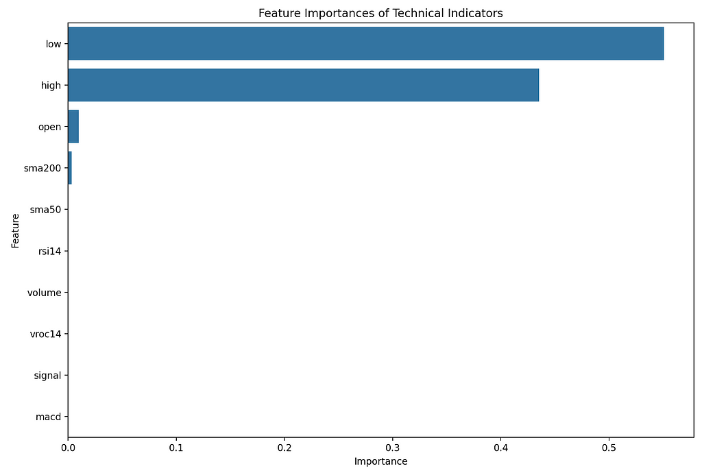Screenshot by Author

Now the way I interpret this is that the technical analysis rules aren’t really being applied, so the features on their own are pretty meaningless.

I’ll give you some examples…

SMA200 and SMA50 on their own doesn’t tell you much, but using the crossovers for buy and sells signals would. Creating feature that shows then the SMA50 is above or below the SMA200 and when it crosses over could be a better feature to feed in.
RSI14 on it’s own doesn’t tell you much. If you used the rules if the RSI14 is below 30 then buy or above 70 then sell then maybe this would be a better feature to track.
MACD and Signal can be very powerful but when you use the crossovers. When the Signal is above and below the MACD. On their own they don’t tell you very much.
VROC14 is also really interesting but again you need to apply some technical analysis rules to understand the buy and sell signals.

I would say with some feature engineering and to take the technical indicators and create features with the buy and sell signals, you would get a much better response.

I will leave that up to you to experiment with :)

Hint: I’ve done this feature engineering in my other articles if you feel like sneaking a peek.

I hope you found this article interesting and useful. If you would like to be kept informed, please don’t forget to follow me and sign up to my email notifications.

If you liked this article, I recommend checking out EODHD APIs on Medium. They have some interesting articles.Michael Whittle

If you enjoyed this, please follow me on Medium
For more interesting articles, please follow my publication
Interested in collaborating? Let’s connect on LinkedIn
Support me and other Medium writers by signing up here
Please don’t forget to clap for the article :) ← Thank you!

Artificial Intelligence (AI) models for Trading was originally published in Coinmonks on Medium, where people are continuing the conversation by highlighting and responding to this story.

Feed: Artificial Intelligence in Coinmonks on Medium

View: Original article

Tags: new testing

Tools And Technologies